Next: Experiments Up: Classifiers used Previous: k-NN The Contents Index
Let us assume we have sets ![]() , these represent
, these represent ![]() classes, each containing
classes, each containing ![]() elements (
elements (![]() ).
We are trying to reduce the dimensionality of input data vectors
).
We are trying to reduce the dimensionality of input data vectors
![]() is
is ![]() to dimensionality
to dimensionality ![]() , where we
believe the classification will be more straightforward, maybe possible using linear classifier. We want to do the following
transformation:
, where we
believe the classification will be more straightforward, maybe possible using linear classifier. We want to do the following
transformation:
Fisher's Linear Discriminant is trying to maximize the ratio of scatter between classes to the scatter within classes.
Two Classes Classification
First let us illustrate this problem in two classes problem. We can see
on figure 3.14 on page ![]() that the projection on vector
that the projection on vector ![]() gives us a chance to find some threshold suitable
for distinguishing whether a potential test sample belongs to class
gives us a chance to find some threshold suitable
for distinguishing whether a potential test sample belongs to class ![]() or
or ![]() . This could be possible because
the projection of
. This could be possible because
the projection of ![]() and
and ![]() on
on ![]() results in two separate sets. While on figure 3.15 on page
results in two separate sets. While on figure 3.15 on page ![]() this is not possible
because the projected class points from
this is not possible
because the projected class points from ![]() overlap with projected class points from
overlap with projected class points from ![]() . We can see that some projections
on vector 1D space are better here and some are worth.
. We can see that some projections
on vector 1D space are better here and some are worth.
![\includegraphics[width=80mm,height=60mm]{lda-intro-twoclasses.eps}](img137.png) |
Now take a look at this in more detail. Assume we are trying to project
sample ![]() , to scalar value
, to scalar value ![]() which corresponds to the metrics of vector
which corresponds to the metrics of vector ![]() , we
are projecting on. This is done by using the
following scalar product:
, we
are projecting on. This is done by using the
following scalar product:
| (3.5) |
It is straightforward that if
![]() is the mean vector for class
is the mean vector for class ![]() , then its projection on vector
, then its projection on vector ![]() is:
is:
The same rule is valid for the scatter. if
![]() is the scatter matrix for class
is the scatter matrix for class ![]() , then
, then
![]() is
scatter projected on
is
scatter projected on ![]() :
:
What we want to do is:
We can see figure 3.16 on page ![]() that
that ![]() does this for us:
does this for us:
![\includegraphics[width=80mm,height=60mm]{lda-intro-twoclasses-mu.eps}](img147.png) |
We can define the criterion for vector ![]() :
:
We want such a ![]() to maximize the function
to maximize the function ![]() .
.
Now we can define scatter matrices. First define scatter within classes matrix:
where
![]() is defined as:
is defined as:
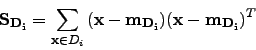
We can easily see that:
We define scatter within classes as the sum of all class scatters. We are trying to find a projection
where these scatters are as small as possible (see figure 3.16 on page ![]() ). This is done by
). This is done by
![]() .
.
We define scatter between classes for two classes (we will change its definition later in Multiple Classes Classification as:
This defines the distance between means of class ![]() and class
and class ![]() . We are trying to find a projection where
this is as distant as possible (see figure 3.16 on page
. We are trying to find a projection where
this is as distant as possible (see figure 3.16 on page ![]() ).
This is done by
).
This is done by
![]() .
.
The maximization of mean distances and minimization of class scatters is done by maximizing ![]() which
we can now rewrite as:
which
we can now rewrite as:
In fact equations (3.8) and (3.6) are the same.
Multiple Classes Classification
As stated in (3.4) FLD does the dimensionality reduction for us. In multiple classes classification
we want to project to space ![]() , where
, where ![]() is the number of classes we have:
is the number of classes we have:
![]() .
.
We will leave the definition of ![]() unchanged but we have to change the definition of
unchanged but we have to change the definition of ![]() . We will define
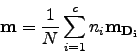
total mean as:
. We will define
total mean as:
which is in fact center of gravity of all class means
![]() and if the mean is computed
using the proper statistic3.1
and if the mean is computed
using the proper statistic3.1
![]() is the center of gravity of all
is the center of gravity of all
![]()
Then we can define scatter between classes as:
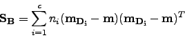 |
(3.10) |
Now what we are going to do is:
| (3.11) |
where ![]() is a projection of
is a projection of ![]() in
in ![]() space,
space,
![]() and
and ![]() is matrix of
is matrix of ![]() x
x ![]() .
.
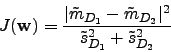
We are trying to maximize ![]() defined very similarly to (3.8):
defined very similarly to (3.8):
As we can see on figure 3.17 on page ![]() LDA transformation is trying to spread classes across
LDA transformation is trying to spread classes across ![]() .
.
Solving Fisher's Discriminator
We can mark ![]() as columns of
as columns of ![]() in (3.12). Then we need to solve the generalized eigenvalue problem:
in (3.12). Then we need to solve the generalized eigenvalue problem:
| (3.13) |
The is the same as:
| (3.14) |
We can use this by Singular Value Decomposition which is implemented in many mathematical programs and libraries.
Once we have the projection matrix ![]() we can do the classification in space of
dimension
we can do the classification in space of
dimension ![]() by projecting test sample to this space and finding the maximum for
by projecting test sample to this space and finding the maximum for
![]() . Another approach can be using Nearest Neighbor in this reduced space.
. Another approach can be using Nearest Neighbor in this reduced space.
Implementation
We can use svd(inv(Sw)*Sb) function implemented in Matlab or PDL::MatrixOps or ccmath. When using Matlab we can also use eig(Sw,Sb) function which can solve the generalized eigenvalue problem.
Possible Issues
The main issue here is that
![]() can be singular when we have a high-dimensional data
(which is usually true for images)
and not enough train data supplied. E.g. in our case we have 32 SIFT tiles each has 9 bins which is in result a vector of dimension 288.
Thus
can be singular when we have a high-dimensional data
(which is usually true for images)
and not enough train data supplied. E.g. in our case we have 32 SIFT tiles each has 9 bins which is in result a vector of dimension 288.
Thus ![]() and
and ![]() are matrices
are matrices ![]() x
x![]() . In an ideal case we would need
. In an ideal case we would need ![]() of train pictures[6] to not have
of train pictures[6] to not have
![]() degenerated.
degenerated.
The possible solution is to use Principal Component Analysis(PCA) first[5,6,7], but the problem is that vectors containing a very important information could be part of PCA null space3.2[5,6].
Kocurek 2007-12-17
![\includegraphics[width=80mm,height=60mm]{lda-intro-twoclasses2.eps}](img138.png)
![\includegraphics[width=80mm,height=60mm]{lda-multi.eps}](img175.png)