Features extraction

Orientation and gradient assignment

We start with orientation $\phi(x,y)$ and gradient $g(x,y)$ assignment for every pixel $(x,y)$ in sample image $I$. Let $I(x,y)$ is a pixel intensity at position $(x,y)$ in image $I$:

• $\forall (x,y) \in I:$ $d_y= (I_{x-1,y-1} + 2I_{x,y-1} + I_{x+1,y-1}) - (I_{x-1,y+1} + 2I_{x,y+1} + I_{x+1,y+1})$ $d_x= (I_{x+1,y-1} + 2I_{x+1,y} + I_{x+1,y+1}) - (I_{x-1,y-1} + 2I_{x-1,y} + I_{x-1,y+1})$ $\phi^{*}(x,y) = \arctan d_y/d_x$ $g(x,y) = \sqrt{d^2_y + d^2_x}$

We would like to obtain the same features for image (a) and (b) in figure 3.6 on page . We need this this result since we want to cope with various metal surface colors from dark colors to bright colors. This is the reason we assign to $\phi(x,y)$ the orientation modulo $\pi$:

$$\phi(x,y) = \pi + \phi^*(x,y) \pmod \pi$$

Figure 3.6: obtained orientation is modulo $\pi$ to obtain the same results for (a) and (b)

The local image descriptor representations

The previous orientations have assigned an orientation and gradient for every pixel in the image. The next step is to compute the descriptor which is distinctive yet is as invariant as possible to parameters such as change in illumination, shift in vertical or horizontal direction or viewpoint change. One usual approach would be to sample local image intensities around the keypoint at appropriate scale and to match these using a normalized correlation measure. However, simple correlation of image patches is highly sensitive to changes that cause misregistration of samples, such as affine or 3D viewpoint change.

As we can see on figure 3.7 on page the image is divided into several square patches (tiles). Every square patch is divided into certain number of bins. Every bin represents a certain interval of orientations which are assigned to it. We call this interval a direction. We can number bins from $1$ to $b$, where $b$ is the number of bins for each tile (i.e. number of directions for each tile). Similarly we can number tiles from $1$ to $t$, where $t$ is the number of tiles.

Figure 3.7: Features Extraction

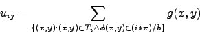
How the values are assigned to every bin depends on the SIFT representation. We proposed 3 variants:

SIFT-Ori

This is the easiest representation. Every orientation has the same vote, which equals to one. Given the $i$-th tile $T_i$ we can compute values for every $j$-th bin as:

$$\forall (x,y)\in T: u_{ij} = \vert\{(x,y): (x,y) \in T_i \wedge \phi(x,y) \in (j*\pi)/b \}\vert$$

where $i$ ranges from $0$ to $b-1$.

With this approach we can have problems when there is the same probability for the direction in the tile. This can apply for random texture but also for circle-like shapes. If we want to distinguish between these two cases we should use votes based on gradient magnitude (SIFT-Grad).

Figure 3.8: Possible distinction between random texture and circle-like shapes

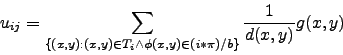
SIFT-Grad

This can be more distinctive between the random textures and circle-like shapes (figure 3.8 on page ). Random textures have usually small local gradients. We can use this information to achieve the similar result as displayed in the picture. We do not want the histograms to be the same (as they would be when each direction has the same vote weight). We can choose the vote weight correlated to the gradient magnitude. Given a tile $T_i$ we have:

$$u_{ij} = \sum_{\{(x,y): (x,y) \in T_i \wedge \phi(x,y) \in (i*\pi)/b\}}{g(x,y)}$$

SIFT-GradWei

This representation can deal better with shifts of the tile. Given the $i$-th tile $T_i$ and $c_x$, $c_y$ is the center of the tile:

$$u_{ij} = \sum_{\{(x,y): (x,y) \in T_i \wedge \phi(x,y) \in (i*\pi)/b\}}{{1\over d(x,y)}g(x,y)}$$

where $d(x,y)$ is computed as:

$$d(x,y)=\sqrt{(x-c_x)^2 + (y-c_y)^2}$$

$d(x,y)$ is the distance of point $(x,y)$ from the center.